Overview
This project builds intuition for spatial filtering and frequency-domain thinking. In Part 1, I compare raw finite differences vs. Gaussian-smoothed derivatives and visualize gradient orientations in HSV. In Part 2, I implement unsharp masking, create hybrid images (high+low frequency fusion), construct Gaussian/Laplacian stacks, and reproduce multi-resolution blending (“oraple”) with both straight and irregular masks.
Part 1 · Fun with Filters
1.1 · Convolutions from Scratch (NumPy-only)
Implemented 2D convolution with a 4-loop naive method and a 2-loop slice-based method,
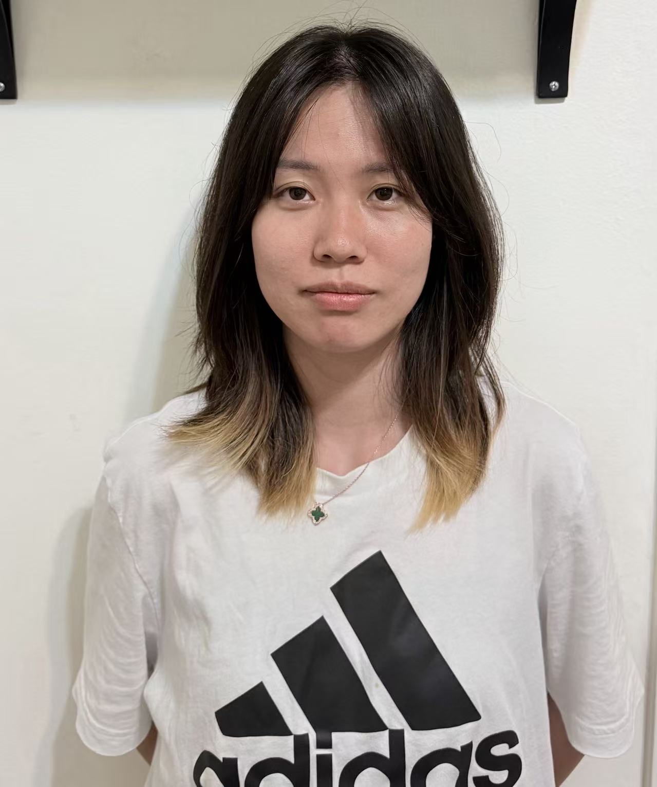
and compared against scipy.signal.convolve2d. Applied a 9×9 box filter on a selfie
(myPic.jpg).


convolve2dCode Snippets
4-loop convolution
def conv2d_4loop(img, kernel):
              H, W = img.shape
              kh, kw = kernel.shape
              pad_h, pad_w = kh // 2, kw // 2
              k = np.flipud(np.fliplr(kernel))  # true convolution (flip kernel)
              padded = np.pad(img, ((pad_h, pad_h), (pad_w, pad_w)), mode="constant")
              out = np.zeros_like(img, dtype=np.float64)
              for i in range(H):
                  for j in range(W):
                      acc = 0.0
                      for u in range(kh):
                          for v in range(kw):
                              acc += padded[i+u, j+v] * k[u, v]
                      out[i, j] = acc
              return out
2-loop convolution
def conv2d_2loop(img, kernel):
              H, W = img.shape
              kh, kw = kernel.shape
              pad_h, pad_w = kh // 2, kw // 2
              k = np.flipud(np.fliplr(kernel))
              padded = np.pad(img, ((pad_h, pad_h), (pad_w, pad_w)), mode="constant")
              out = np.zeros_like(img, dtype=np.float64)
              for i in range(H):
                  for j in range(W):
                      region = padded[i:i+kh, j:j+kw]
                      out[i, j] = np.sum(region * k)
              return out
SciPy + save & diffs
# 9×9 box filter
          box9 = np.ones((9, 9), dtype=np.float64) / 81.0

          img = load_image_gray("../data/myPic.jpg")
          out_4loop = conv2d_4loop(img, box9)
          out_2loop = conv2d_2loop(img, box9)
          out_scipy = convolve2d(img, box9, mode="same", boundary="fill")

          # rotate 90° clockwise for display
          plt.imsave("../out/11/box9_4loop.jpg", rot90_cw(np.clip(out_4loop, 0, 1)), cmap="gray")
          plt.imsave("../out/11/box9_2loop.jpg", rot90_cw(np.clip(out_2loop, 0, 1)), cmap="gray")
          plt.imsave("../out/11/box9_scipy.jpg", rot90_cw(np.clip(out_scipy, 0, 1)), cmap="gray")

          # absolute-diff heatmaps vs SciPy
          eps = 1e-12
          diff_4 = np.abs(out_4loop - out_scipy); d4 = diff_4 / (diff_4.max() + eps)
          diff_2 = np.abs(out_2loop - out_scipy); d2 = diff_2 / (diff_2.max() + eps)
          plt.imsave("../out/11/diff_4loop.jpg", rot90_cw(d4), cmap="inferno")
          plt.imsave("../out/11/diff_2loop.jpg", rot90_cw(d2), cmap="inferno")
Conclusion. My 4-loop and 2-loop implementations numerically match the SciPy baseline (toggle to view Δ heatmaps). The 9×9 box filter blurs the image, confirming its low-pass nature: it removes high-frequency details and preserves smooth low-frequency content.
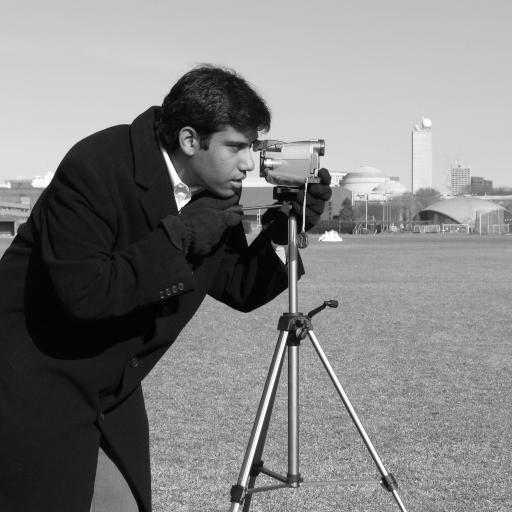
1.2 Finite Difference Operator
Dx=[-1,1], Dy=[-1;1] on cameraman; gradient magnitude and thresholded edges (manual τ).
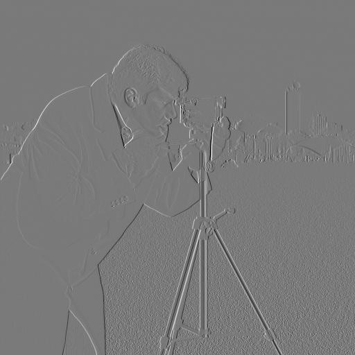
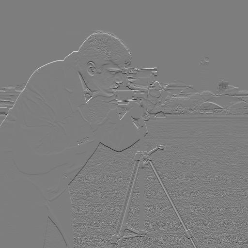
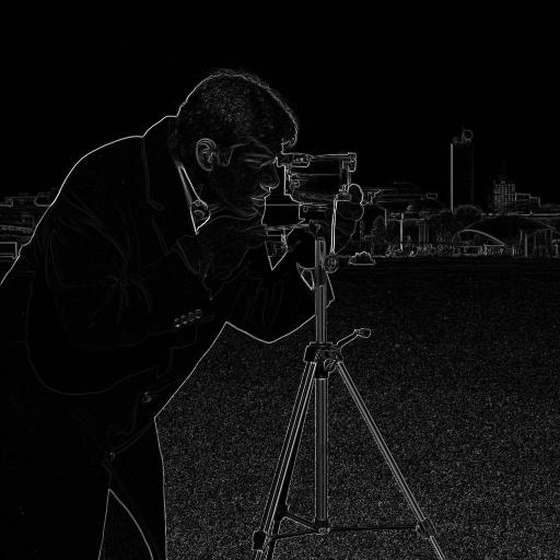
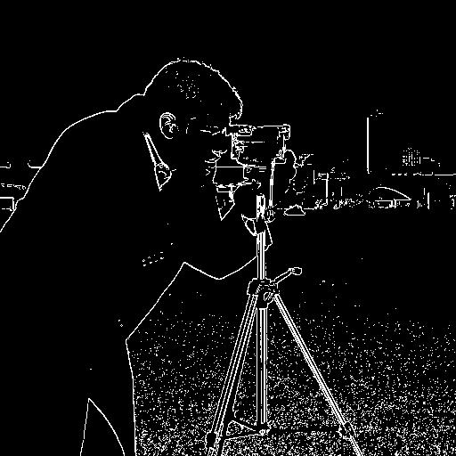
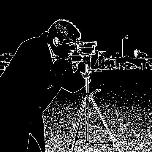
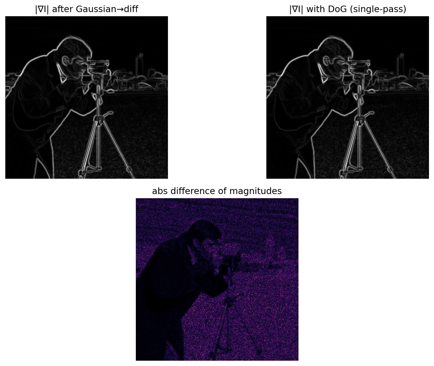
1.3 Derivative of Gaussian (DoG)
Gaussian pre-smoothing reduces noise. DoG (Gaussian ⊗ D) produces smoother edges than raw finite differences, and matches the two-stage blur→difference pipeline in one pass.
Part 2 · Fun with Frequencies
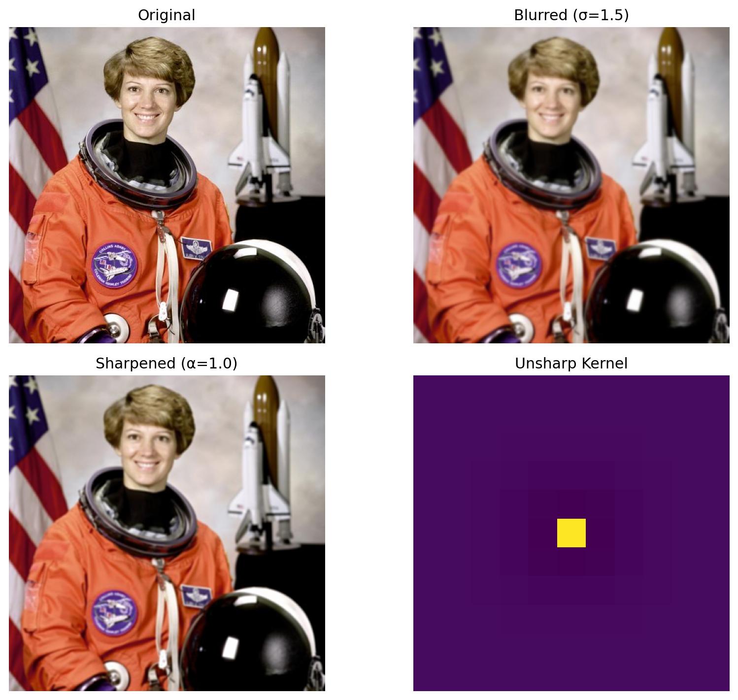
2.1 Image “Sharpening” (Unsharp Mask)
Low-pass with Gaussian → subtract to get high-freq → add scaled high-freq (α) back. Also: blur a sharp image then try to “restore” via unsharp; discuss what cannot be recovered.

2.2 Hybrid Images
Align two images; low-pass one, high-pass the other; add. Show log-magnitude FFTs of inputs, filtered, and hybrid. Include 2–3 creative pairs; experiment with color vs grayscale.
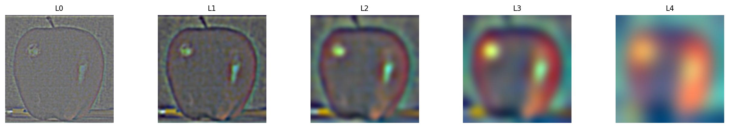
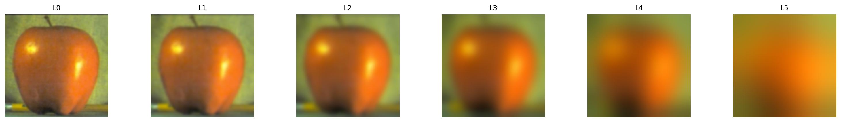
2.3 Gaussian & Laplacian Stacks
Same-size stacks (no downsampling): Gaussian at increasing σ; Laplacian as difference of adjacent Gaussian levels + coarsest residual. Visualize per level to inspect band-limited content.
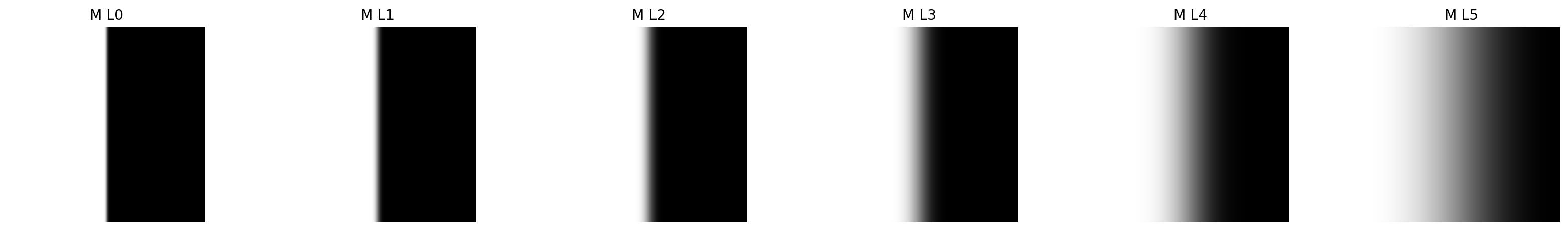
2.4 Multi-resolution Blending (Oraple)
Build Laplacian stacks for A/B and a Gaussian mask stack; blend per level
Fi = Mi·LAi + (1−Mi)·LBi; reconstruct by summing levels (stack variant).
Show straight seam and irregular masks; include level visualizations like Fig. 10.

Discussion
Observations, failures, parameters, runtime
- DoG substantially suppresses noise vs. raw finite differences; orientation-HSV makes edge flow intuitive.
- Unsharp exaggerates ringing if α or σ is too large; true lost detail (from blur) cannot be fully restored.
- Hybrid images depend critically on alignment and cutoff choices (σlow, σhigh).
- Stack blending with a Gaussian mask stack removes seams; irregular masks produce more natural composites.
- Runtime is fast with vectorized
convolve2d; stack levels (no downsampling) simplify visualization.